Model framework to evaluate the suitability of groundwater regime for crop growth
Introduction
The main objective of this project is to determine the impact of the groundwater levels on common crops in Flanders. The model instruments used in this study are the same as those behind the Dutch initiative WaterVision Agriculture: the soil water transport model SWAP coupled to the crop model WOFOST. The coupled instrument does not only take into account drought stress on plants, but also oxygen stress under too wet conditions. In addition, indirect effects affecting sowing, mowing or harvest times can be quantified.
SWAP-WOFOST has been extensively verified in the last decades. The numerical solutions of SWAP were also compared with analytical solutions. An overview of some validation and sensitivity analysis cases can be found in Heinen et al. (2021). Since the start of the WaterVision Agriculture tool in 2015, the model instruments were continuously developed and improved. A recent validation at regional and local scale for grass and silage maize satisfactorily compared the simulated crop development and transpiration reduction with observed NDVI values Mulder et al., 2021.
Since the model has been extensively tested in fairly similar Dutch conditions, we focused on adapting the input data to Flemish conditions (weather, soil and groundwater level) and on validating the simulated yields with historic local yield data from various trials. Crop parameters were thereby not altered. The information on the model framework is largely extracted from the SWAP-WOFOST manual Kroes et al., 2017 and related articles Werkgroep Waterwijzer Landbouw, 2018. More information can be found in those sources.
The SWAP-WOFOST model
SWAP (Soil, Water, Atmosphere and Plant) is a one-dimensional, field scale and vertically directed model that simulates the transport of water, solutes and heat in the unsaturated and saturated zone, in interaction with vegetation development Kroes et al., 2017Dam et al., 2008. SWAP allows to consider water exchange with the surroundings, like discharge to ditches, drains and other surface waters. The crop growth module WOFOST (World Food Studies; De Wit et al. (2020)) is integrated in SWAP to describe the phenological development, growth and yield production of major arable crops.
The main input information consists of weather data, groundwater levels and soil & crop characteristics. The model output comprises time series of water (and solute) balances and crop dry matter development. In addition, the occurrence of different stress types over the growing season is quantified.
SWAP-WOFOST was developed in The Netherlands by Wageningen University and Research and is freely available in https://
Soil water transport
SWAP Kroes et al., 2017 computes transport of water, solutes and heat in the unsaturated and saturated zone using Richards equation, including root water extraction to simulate the movement of soil moisture in variably saturated soils. The SWAP domain is considered from just above the canopy of the crop to a plane in the phreatic groundwater (Figure 1). In this domain, the transport processes are predominantly vertical. Below the phreatic groundwater level (saturated zone), the model can also estimate lateral drainage fluxes. However, this option was not activated in this project. SWAP can simulate discharge to ditches, drains and other surface waters, through drainage and infiltration equations acting as sinks or sources in the 1-D model, completing the vertical water balance.
The top boundary conditions of the system are characterized by the soil surface with or without vegetation and the atmospheric conditions. The bottom boundary condition describes the interaction between saturated shallow soil layers with regional groundwater, while the lateral boundary explains the interaction with surface water systems (Figure 1).
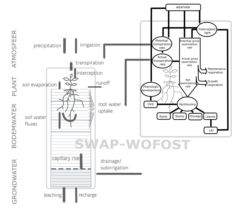
Figure 1:Schematic representation of the functioning of the coupled SWAP-WOFOST model (1-D) used for this study.
The major concepts and assumptions of SWAP-WOFOST used in this study include Heinen et al., 2021:
- The evaporation demand of the atmosphere is calculated using the Penman-Monteith equation Monteith, 1965.
- The water movement is vertical (one-dimensional model) and described by the Richards equation.
- Water retention characteristics of each soil layer are described with Mualem-Van Genuchten functions.
- The porous medium is assumed to be rigid, isotropic and isothermal.
- Soils can be variably saturated and heterogeneous.
- The bottom boundary conditions can be specified as flux or pressure head, and may depend on the phreatic groundwater, or the hydraulic head in the deeper aquifer and resistance of the system.
- Transpiration reduction can be caused by very dry conditions (water stress), very wet conditions (oxygen stress). Salinity stress was not considered.
- Ponding occurs when the soil infiltration capacity is exceeded, and surface runoff takes place only after a threshold ponding height is surpassed (i.e. 0.2 cm).
- Soil temperature is simulated as a diffusion process.
- Irrigation can be considered as fixed applications or chosen according to irrigation criteria. Irrigation was not considered in this study.
The Richards equation for variably saturated soils ( (1)) is solved numerically in SWAP for every soil compartment, using specified boundary conditions and relations between θ, h and K, given by the Mualem-Van Genucthen functions:
In (1), θ is the volumetric water content (cm3 cm-3), t is time (d), K(h) is the hydraulic conductivity (cm d-1), h is the soil water pressure head (cm), z is the vertical coordinate (cm) taken positive upward. is the soil water extraction rate by roots (cm3cm-3 d-1), is the extraction rate by drain discharge in the saturated zone (cm3cm-3 d-1) and is the exchange rate with macro pores (cm3cm-3 d-1).
In this study, the only sink term considered is the soil water extraction rate by roots ().
Bottom boundary conditions
The bottom boundary is located in the unsaturated zone or in the upper part of the groundwater table. The bottom boundary condition can be determined by an imposed pressure head (e.g. groundwater level), an imposed water flux (e.g seepage ) or a combination of the two (e.g. q-H relation), depending on the application and spatial scale. In total, SWAP offers eight options to prescribe the bottom boundary condition. Option 5 “Prescribed soil water pressure head of bottom compartment” was chosen in this study.
For the selected bottom boundary condition, the pressure head at the bottom of the soil profile (bottom compartment) and date must be specified. For times between observations, SWAP interpolates linearly.
Crop growth
The dynamic crop growth model WOFOST De Wit et al., 2020, integrated in SWAP, describes the phenological development, growth and yield formation of major arable crops. The potential transpiration and yield are determined by the incoming radiation, carbon dioxide concentration, air temperature and crop characteristics. The actual transpiration and yield are calculated based on the decreased crop water uptake due to drought and/or lack of oxygen, as calculated by SWAP.
WOFOST calculates how much light and CO2 is intercepted and potentially converted by photosynthesis. The actual photosynthesis is then calculated by reducing the potential photosynthesis for limited availability of moisture for evaporation or oxygen deficiency. Part of the energy produced during photosynthesis is used for maintenance respiration, and other part is converted into dry matter. During this conversion, some energy is lost as growth respiration. The dry matter produced is distributed over the different parts of the crop: roots, stems, leaves and storage organs, depending on temperature and the development stage of the crop. Some simulated crop growth processes like the maximum rate of photosynthesis and the maintenance respiration, are influenced by temperature. Other processes like the distribution of assimilates or senescence of crop tissue are controlled by the phenological stage of the crop. The phenological development stage also depends on temperature.
A dynamic grass growth model “GRASS”, derived from WOFOST, is specifically developed for the simulation of grassland Kroes & Supit, 2011, to consider the differences in the growing stages and cultivation practices between grass and arable crops. Grass is perennial and remains in the vegetative period during most of its growing season. Also, it is frequently mowed or grazed. Mowing and grazing in the model occur when the above ground dry matter exceeds a certain threshold ( value). Grass is simulated as a permanent grassland, and five combinations of mowing and grazing management scenarios are available. In practice, the time of mowing/grazing will depend on the farm management and interaction between different fields. This grass module is experimental and calibrated for Dutch conditions, but several studies have shown its robustness Mulder et al., 2021.
Direct and indirect effects
Yield reduction due to changes in hydrological conditions distinguishes between direct and indirect effects. Direct effects are linked to water and oxygen stress ( and salinity stress), while indirect effects are related to how prevailing hydrological conditions affect sowing and harvesting.
Direct effects on yield
Sub-optimal soil moisture conditions (too wet or too dry) have a direct influence on the yield of agricultural crops. Under these conditions, crop transpiration is reduced due to stomatal closure. This also reduces the absorption of CO2, leading to less photosynthesis and less growth.
To determine the uptake of water by plant roots, SWAP first calculates the potential transpiration (i.e. the transpiration at optimal soil moisture conditions). This is calculated based on weather variables (solar radiation, air temperature, humidity and wind speed) and plant characteristics (crop height, reflection coefficient, leaf area index and minimal stomatal resistance). The potential transpiration is distributed over the root zone, proportional to the root density, to determine the potential uptake of water by the roots. Then, based on the soil moisture conditions at different depths in the root zone, the extent of damage due to dry or wet conditions is determined. SWAP uses stress factors (0 - 1) for every sub-optimal condition, at each soil compartment, to calculate the actual plant root water uptake.
and are the stress factors for too dry and too wet conditions, respectively. is the potential root water uptake, is the actual root water uptake at each soil compartment, and is the actual transpiration over the entire root zone, or in other words, the sum of individual root water uptakes multiplied by the compartment thickness. The transpiration reduction due to each stress is calculated by multiplying the total reduction in crop water uptake with the proportion of the logarithmic value of the corresponding stress factor ((4)).
It is assumed that the relative distribution in transpiration reduction is equal to the relative yield loss.
Drought stress
Drought stress is calculated by the function of Feddes et al. (1978) (Figure 2). Above , root water uptake is optimal and no drought stress occurs. Below , the root water uptake linearly decreases until zero at (wilting point). Generally, fixed values for h3 and h4 are used. However, the drought stress threshold () depends on crop type, soil texture, root density and atmospheric demand, and the linear decline may deviate from reality. Therefore, a detailed, microscopic root water uptake module for drought has been added in SWAP Lier et al., 2013 and can be chosen as alternative to Feddes et al. (1978).
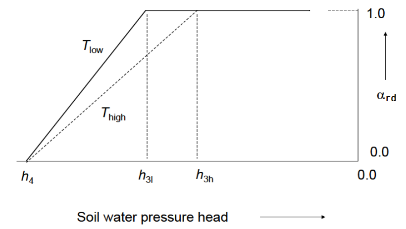
Figure 2:Reduction factor for root water uptake, , as function of soil water pressure head (h) and potential transpiration rate () Feddes et al., 1978
Oxygen stress
Oxygen stress influences crop yield via the aeration of the soil, whereby the oxygen supply to plant roots takes place. Under too wet conditions, air in the soil pores is replaced by water and the availability of oxygen becomes limiting for root respiration. Root respiration is determined by the transport of oxygen in the soil and the demand by the roots. Since the transport of gas in water-filled pores is approximately 1000 times lower than that in air-filled pores, the availability of oxygen is determined by the air content at the different soil depths (Figure 3). In addition to respiration by roots, the available oxygen is used for respiration by microorganisms. The link with the crop growth model WOFOST makes it possible to describe the oxygen demand of plant roots in detail.
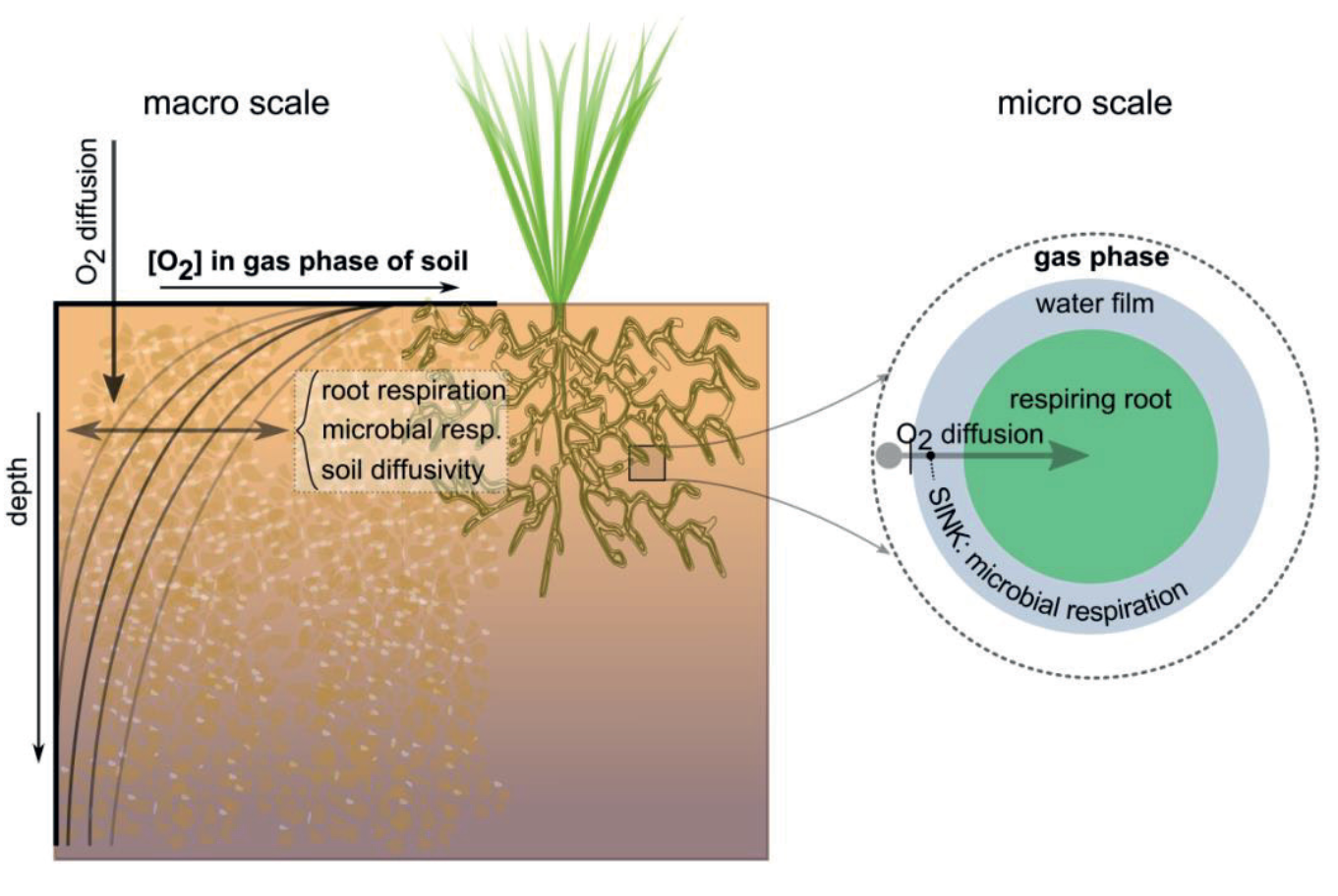
Figure 3:Schematization of the oxygen module for determining daily respiration and transpiration reduction. The module combines physiological processes, root and microbial respiration; and physical processes, diffusion at both macro and microscale. Figure taken from Bartholomeus et al. (2011).
Oxygen transport is calculated in SWAP using the model proposed by Bartholomeus et al. (2008). In this model, the critical gas filled porosity for oxygen stress depends on several abiotic (soil physical properties, moisture content, temperature) and biotic factors (plant characteristics). Therefore, the model of Bartholomeus et al. (2008) is applied for every soil layer, to calculate the difference between potential and actual root respiration and subsequently, the reduction factor due to oxygen stress (wet conditions).
Indirect effects on yield
In SWAP, indirect effects refer to restrictions in normal agricultural practices due to too wet or too cold conditions, which ultimately shortens the growing season. These include limited carrying capacity for tillage, sowing/planting or harvesting, delayed germination, and crop damage Werkgroep Waterwijzer Landbouw, 2018. Other indirect effects like quality of harvest, soil quality, pests and diseases are not taken into account. More context about different indirect effects can be found in the chapter Impact of groundwater levels and waterlogging on cultivation factors. Indirect effects like pests and diseases along with nutrient deficiency are accounted for in one single management factor “RELMF”, which varies with the type of crop. These factors were obtained from several experiments under Dutch conditions and double-checked by plant scientists, for the WaterVision Agriculture tool, which were maintained in this study. Nutrient deficiency during the growing period is not implemented in this version of the model, but a nitrogen module is available Groenendijk et al., 2016.
For arable crops, different machinery is used for preparatory works (i.e. tillage), sowing or planting, and harvesting. The start of each of these stages can be delayed if the soil is too wet for the machines to enter the field, or too cold for the seed to germinate. In the model, this is determined based on a pressure head criterion derived from Beuving (1982), and a temperature criterion in case of germination (temperature sum needed for crop emergence). A certain pressure head, at 15 cm depth, has to be met before preparation works, sowing or harvesting can start, which depends on soil and crop characteristics. WaterVision Agriculture distinguishes between two categories for the pressure head criterion: light and heavy. This is a weight category that depends on the weight of the most common machine used for the specific crop (Table 4.1, 4.2, and 4.4 of Werkgroep Waterwijzer Landbouw (2018)). Plowing, always falls under the heavy category. For sowing, maize and potatoes are in the heavy category, while winter wheat and sugar beet fall in the light category. For harvesting, all the five crops fall in the heavy category.
In grass, indirect effects are related to insufficient carrying capacity for mowing or grazing. In this case, when a certain pressure head, at 15 cm for mowing or at 10 cm for grazing, is exceeded, harvest decreases by a certain percentage based on the degree of exceedance. In this study, only mowing was considered since it is the main grass management in Flanders.
In order to find the pressure head values for the Flemish soils, top soils (first soil layer of each soil profile) were first translated to the Dutch soil classification “The Staring series” Heinen et al., 2020 based on the soil texture and organic matter. Then, the appropriate pressure head was assigned to every soil profile and crop. Table 1 presents the different pressure head thresholds used for the Flemish soil types, according to the light and heavy category. This is a rather simple method but allowed to include approximated pressure head values in the model, and calculate indirect effects.
Table 1:Pressure head criterion at 15 cm depth according to light and heavy category, for different soil types in Flanders. Values are taken from Table 4.1 of Werkgroep Waterwijzer Landbouw (2018).
Staring building block | Description | Soil Belgian classification | Preparatory works | Pressure head at 15 cm depth (cm) Light category | Pressure head at 15 cm depth (cm) Heavy category |
|---|---|---|---|---|---|
B01- B04 | Weakly loam to very strong loam with very fine to moderately fine sand | sand (Z) loamy sand (S) light sandy loam (P) sandy loam (L) | spring | -50 | -60 |
B07 | Very light sludge | light sandy loam (P) loamy sand (S) sandy loam (L) loam (A) | autumn | -60 | -60 |
B08 | Moderately light loam | sandy loam (L) loam (A) | autumn | -60 | -90 |
B09 | Heavy sludge | loam (A) clay (E) | autumn | -60 | -90 |
B10-B12 | Light to very heavy clay | clay (E) heavy clay (U) | autumn | -70 | -100 |
B13 | Sandy loam | sandy loam (L) loam (A) | autumn | -70 | -100 |
B17 | Peaty clay | loam (A) | spring | -60 | -80 |
By taking into account the possibility that the growing season may be shifted or shortened, the model actually introduces a “second” calculated potential crop yield associated with a sub-optimal growing season. Figure 4 illustrates how indirect effects are calculated in the model. In the absence of indirect effects, the situation would be similar to the figure on the left (reference situation), where just direct effects (water and oxygen stress) are considered, and the potential yield () is the maximum possible. After a wetting measure, the situation can become similar to the figure on the right, where indirect effects now play a role and the growing season is shortened. In this condition, this “second” potential yield () and actual yield implicitly include the reduction due to indirect effects. To determine the maximum potential crop yield , the model assumes a deep groundwater level of 5 m to minimize the indirect effects of excessively wet conditions due to shallow groundwater levels. The difference between these potential yields represents the yield reduction due to indirect effects (uaAzsdo81y).
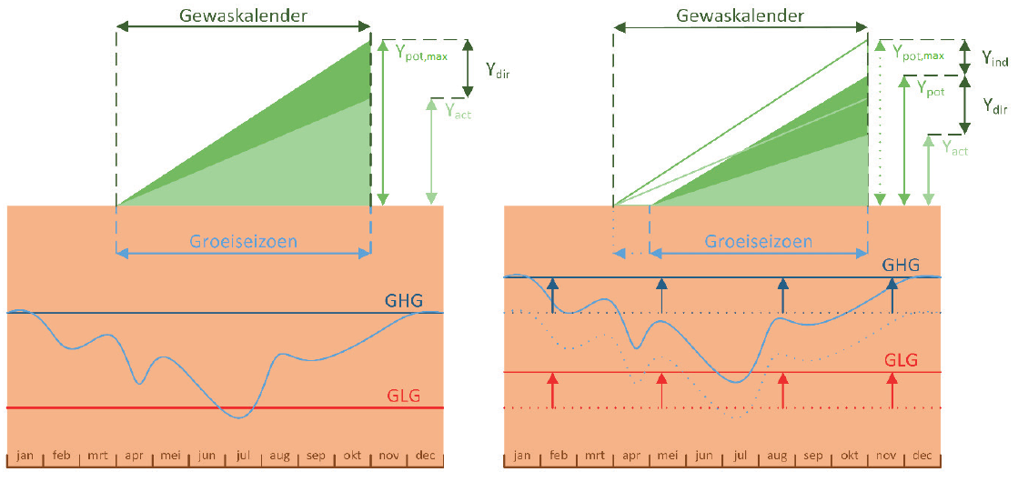
Figure 4:Example of the calculation of the potential and actual yield when taking into account direct and indirect effects. On the left, the reference situation is displayed, and on the right , the situation after a wetting measure. The dark green area represents the potential crop yield and the light green area, the actual crop yield. Figure extracted from Werkgroep Waterwijzer Landbouw (2018).
Yield reduction
The potential crop yield is calculated using the dynamic crop model as function of the CO2 content, solar radiation, temperature, crop characteristics, and based on the pressure head criterion and temperature criterion at the start and end of the growing season. The transpiration reduction due to too dry and too wet conditions is used to calculate the actual crop yield. The total yield reduction () in % is defined as the relative difference between the maximum potential yield () and actual yield () ((6)). The yield reduction due to direct effects is the difference between and ((7)).
The yield reduction due to each stress ( dry or wet conditions) is calculated by multipliying with the proportion of each transpiration reduction, from (4).
The potential and actual crop yield, and transpiration reduction due to each stress were the main model output variables for this study.
Model Input
To get realistic model results, a good estimation of the boundary conditions and soil properties is fundamental. This regional version for Flanders uses freely available datasets and maps for the whole of Flanders (online or on request), obtained from Flemish institutions or from previous projects (Table 2). Despite the inherent limitations of such generic and large-scale data, the information is suitable for applying the model in a regional scale. More detailed information about the different input data layers is given below.
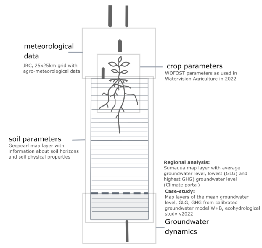
Figure 5:Schematic overview of the information/data used to shape the model parameters and necessary input variables in the model framework of PEILIMPACT. If a user has more accurate data for one or more of these components, they can replace the data layers applied here.
Note: For the case study De Zegge-Mosselgoren (Case-study: agricultural land around De Zegge-Mosselgoren ) this input data (weather data and soil information) was combined with the groundwater levels from a locally calibrated groundwater model (preliminary results) from the “Ecohydrological study: basis for restoration measures for Nature Reserve De Zegge” (Witteveen+Bos) instead of the general map of average groundwater levels used for the regional analysis of Flanders. Unfortunately, this study was very behind schedule, which meant that we were unable to work with the final results of the ecohydrological study and to calculate future scenarios to quantify the effects on agriculture.
Table 2:Overview of the input data used in SWAP-WOFOST
Input data | Description | Source |
|---|---|---|
Meteorological data | Daily interpolated meteorological variables from 01/01/1990 until 31/12/2021, 25 x 25 km resolution. | |
Crop data | Planting and harvesting dates | ILVO and Dutch crop calendar |
Soil data | Soil texture, soil hydraulic parameters and vertical discretization of 536 soil profiles over Flanders. | Flemish Institute for technological Research (VITO), from the GeoPearl model Joris et al., 2017 |
Groundwater levels (GWL) maps (Regional scale) | Average GWL, average highest GWL (GHG) and average lowest GWL (GLG) maps, 100 m resolution. | Effecten van Klimaatverandering op de freatische grondwaterstanden (Sumaqua) Franken & Wolfs, 2022 |
Groundwater levels (GWL) maps (Case study) | Average GWL, average highest GWL (GHG) and average lowest GWL (GLG) maps, 10 m resolution. | “Ecohydrological study: basis for restoration measures for Nature Reserve De Zegge” (Witteveen + Bos) (ongoing study) |
Extra map layers (e.g. provinces, main rivers) were downloaded from The Atlas of Belgium, for graphical purposes.
To link the input data with its corresponding location (i.e. coordinates) in Flanders, ASCII maps were used. These maps were generated in QGIS 3.22, using the Belgian Lambert 72 (EPSG: 31370) projection system. For the regional analysis, the maps were homogenized to 500 m resolution using a simple upscaling criterion, either “mean value” or “majority” in the Resampling tool. For the case study, the original resolution was maintained.
Meteorological data
The Joint Research Center (JRC) contains daily interpolated agro-meteorological data for Europe and neighboring countries, with a 25 km resolution, from 1979 to the last calendar year completed. Up to the date of this project, data from 01/01/1979 until 31/12/2021 is available. Table 3 presents the meteorological information provided in JRC and used in the model. Units conversion and formatting was done before using it in the model.
Table 3:Meteorological variables and their units as given in JRC.
Variable | Units |
|---|---|
Maximum air temperature | °C |
Minimum air temperature | °C |
Mean daily wind speed at 10 m | m s-1 |
Vapour pressure | hPa |
Sum of precipitation | mm d -1 |
Total global radiation | kJ m-2 d-1 |
The meteorological ASCII map was built based on the coordinates ( blue points in Figure 6) of the meteorological grids as given by JRC, and applying voronoi polygons in QGis. In this way, the corresponding region for each point could be determined, which is similar to a grid of 25 km x 25 km resolution (Figure 6). Finally, the map was exported to 500 m resolution.
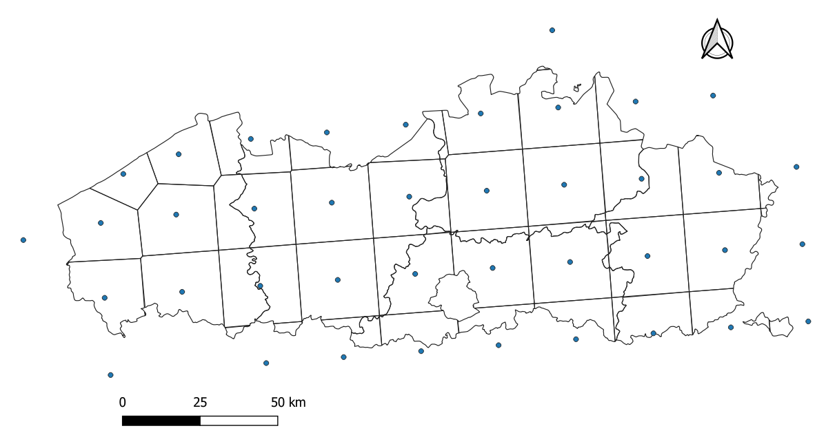
Figure 6:Raster map showing the location of the JRC meteorological grids.
Crop data
Typical planting and harvest dates in Flanders were determined with the help of ILVO experts. These dates are similar to the ones assumed in WaterVision Agriculture. Table 4 shows the growing season for the 5 crops modeled in this study, together with their period of planting, harvesting and mowing (in the case of grass) in Flanders. The dates in the table indicate the planting and harvesting dates used in the model.
Table 4:Crop calendar of the 5 crops simulated with SWAP-WOFOST. Colored cells represent the time span for planting, harvesting and mowing (in case of grass) in Flanders, while the specific dates are the planting and harvest dates used in the model.
Crop | Jan | Feb | Mar | Apr | May | Jun | Jul | Aug | Sep | Oct | Nov | Dec |
|---|---|---|---|---|---|---|---|---|---|---|---|---|
Potato | 15/04 | 01/10 | ||||||||||
Silage maize | 25/04 | 01/10 | ||||||||||
Winter wheat | 20/08 | 10/10 | ||||||||||
Sugar beet | 16/03 | 15/11 | ||||||||||
Grass | 01/01 | 31/12 |
|
|
| Growing season |
| Planting | ||
| Harvesting | ||
| Mowing | ||
Soil data
Soil texture, soil hydraulic parameters and characterization of the soil profiles over Flanders were provided by the Flemish Institute for technological Research (VITO), from the GeoPearl model Joris et al., 2017. There are in total 536 dominant soil units defined over Flanders. Soil texture, organic carbon, and pH for each soil horizon are extracted from the Aardewerk database 2010 VPO, 2011 and the Belgian soil map VPO & IWT, 2014. Soil hydraulic properties are calculated using the extracted soil properties and the pedotransfer functions of Wösten et al. (1999). Soil profiles are defined to a depth of 3 m and subdivided into 5 to 7 horizons. In this study, the depth of the soil profiles was extended to 6 m.
Bulk density (BD) was calculated according to the formula of Vereecken (1988), shown in (9), which depends on the percentage of organic carbon (Corg) . This formula applies for sand (Z), loamy sand (S) and light sandy loam (P) textures. For other textural classes, bulk density is assumed equal to 1.48 g cm-3. This is obviously a simplification of reality. The bulk density in SWAP is especially important for determining the maximum rooting depth of the crops.
Soil texture according to the Belgian Soil Classification system
The soil texture according to the Belgian Soil Classification system Dondeyne et al., 2014Van De Vreken et al., 2009 for each of the 536 soil units, was determined based on the clay and sand content of the first top soil layer. Figure 7 shows the soil textural classes in Flanders according to this classification, based on the soil properties used in the model.
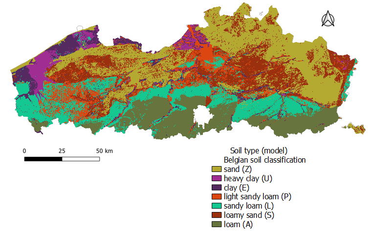
Figure 7:Soil texture according to the Soil Belgian Classification System, based on the textural information used in the model.
This map is less detailed than the Belgian Soil Map since the classification was based just on the clay and sand content of the first layer and mainly serves to visualize trends between crop yield, groundwater and soil types.
Maximum rooting depth allowed by the soil
The maximum rooting depth depends on plant and soil characteristics. Ranges of maximum rooting depth for different crops can be found in the FAO guidelines Allen et al., 1998. We defined the maximum rooting depths for each plant as in the WaterVision Agriculture tool (Table 5), which slightly differ from values provided by the FAO. However, normal root growth can be restricted in the presence of hard soil layers, compaction, and boundaries in the soil (e.g. rocks) Moore et al., 1998. Therefore, root growth restrictions were considered when:
- pH < 4.0
- BD > BD calculated by linear interpolation for its respective clay content, between points: BD = 1.6 g cm-3 and clay = 20 %, and BD = 1.2 g cm-3 and clay = 65 %.
Table 5:Maximum rooting depth according to crop characteristics assumed in the model.
Crop | Maximum rooting depth (cm) |
|---|---|
Potato | 50 |
Silage maize | 100 |
Winter wheat | 125 |
Sugar beet | 120 |
Grass | 40 |
The check of the BD was done for each soil layer and when the BD is exceeded or PH is lower than 4, roots cannot grow deeper, even though this is still theoretically possible. The minimum rooting depth is 10 cm for grass and 20 cm for other crops. If no restrictions were imposed by the soil, the maximum rooting depth would be the one given in Table 5. The spatial variability of the maximum rooting depth allowed by the soil is shown in Figure 8.
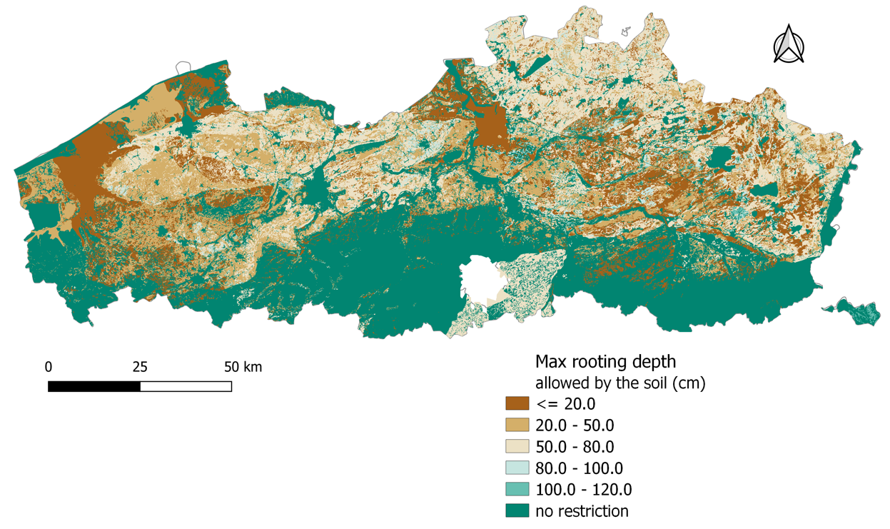
Figure 8:Spatial variation of the maximum rooting depth allowed by the soil as given in the model.
Soil discretization
To get realistic simulations of the water infiltration in the soil matrix, especially at the soil surface, the grid cells or soil compartments for numerical solution of the Richards equation have to be small enough. The SWAP manual Kroes et al., 2017 provides some guidelines to define the thickness of the soil compartments, which are shown in Table 6. The initial discretization from the GeoPearl soil input was therefore adapted to comply with these guidelines.
Table 6:Vertical discretization of the soil profile for numerical solution of Richard’s equation.
Depth of the soil profile (cm) | Compartment thickness (cm) |
|---|---|
0 - 50 | 1 |
50 - 80 | 2 |
80 - 140 | 5 |
140 - 200 | 10 |
200 - 300 | 20 |
300 - 600 | 25 |
Phreatic groundwater levels
Average groundwater levels (Figure 9), and average highest (GHG) and lowest groundwater levels (GLG) maps, with 100 m resolution, were provided by Sumaqua in the context of the project “Actualiseren grondwaterstandsindicator en berekening effecten van klimaatverandering op de freatische grondwaterstanden” Franken & Wolfs, 2022. The average groundwater levels for all pixels were obtained from Machine Learning (ML) trained with a large number of observations in Flanders (5673 locations). The GHG and GLG maps were approximated using ML based on the results of 217 long term SWAP simulations, for points in which some correlation between precipitation and groundwater was observed. GHG & GLG maps do not contain information in the locations closer to watercourses where said correlation does not exist. Note that the generated maps are predictions and are not necessarily valid in locations where drainage or GWL extractions are present without a data point nearby to train the algorithm.
Different natural factors are involved in the groundwater level (GWL) fluctuations and the response time of the groundwater system to a certain precipitation event (time lag). One factor is the cumulative precipitation deficit (precipitation - reference evapotranspiration, P-ET0), which is highly correlated with GWL. However, the time response of the system can vary from less than a month to even years. This time delay is mainly influenced by the depth of the GWL Wossenyeleh et al., 2020Londot & Huysmans, 2021, which also defines how strong the seasonal effects of the precipitation in GWL are. Shallow GWL normally have more correlation with P-ETref than deep GWL. Wossenyeleh et al. (2020) found that in relatively shallow GWL (<10 m), the delay ranges between 0-2 months. In places close to rivers, ditches or drains however, the GWL fluctuations will be more influenced by the surface water levels instead of the P-ET0. Another factor is soil texture, which defines the storage capacity of the soil. Additional to these natural factors, there are also anthropogenic conditions like unknown GWL abstractions and sewers, which also affect the GWL fluctuations.
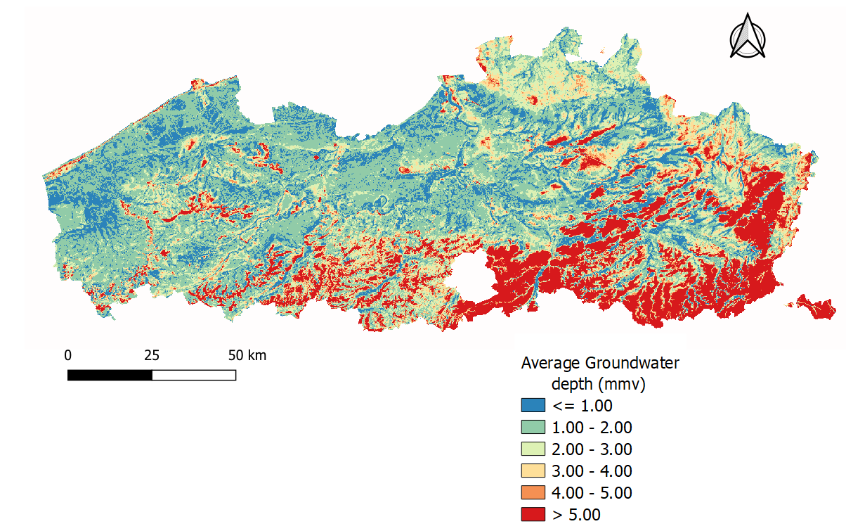
Figure 9:Spatial variation of the groundwater levels in Flanders Franken & Wolfs, 2022
Description of the phreatic groundwater dynamics
The seasonal fluctuations of the GWL are crucial to predict its impact on the growth of arable crops. Yet, the available information in Flanders does not describe these dynamics. In this study, GWL fluctuations were approximated by the sinus function of (11). This sinus curve was calculated in every location and varies according to the average highest (GHG) and lowest groundwater levels (GLG), but keeps constant through the years (Figure 10). The shape of the curve is based on the monthly P-ET0 over Flanders for the period 1979-2021.
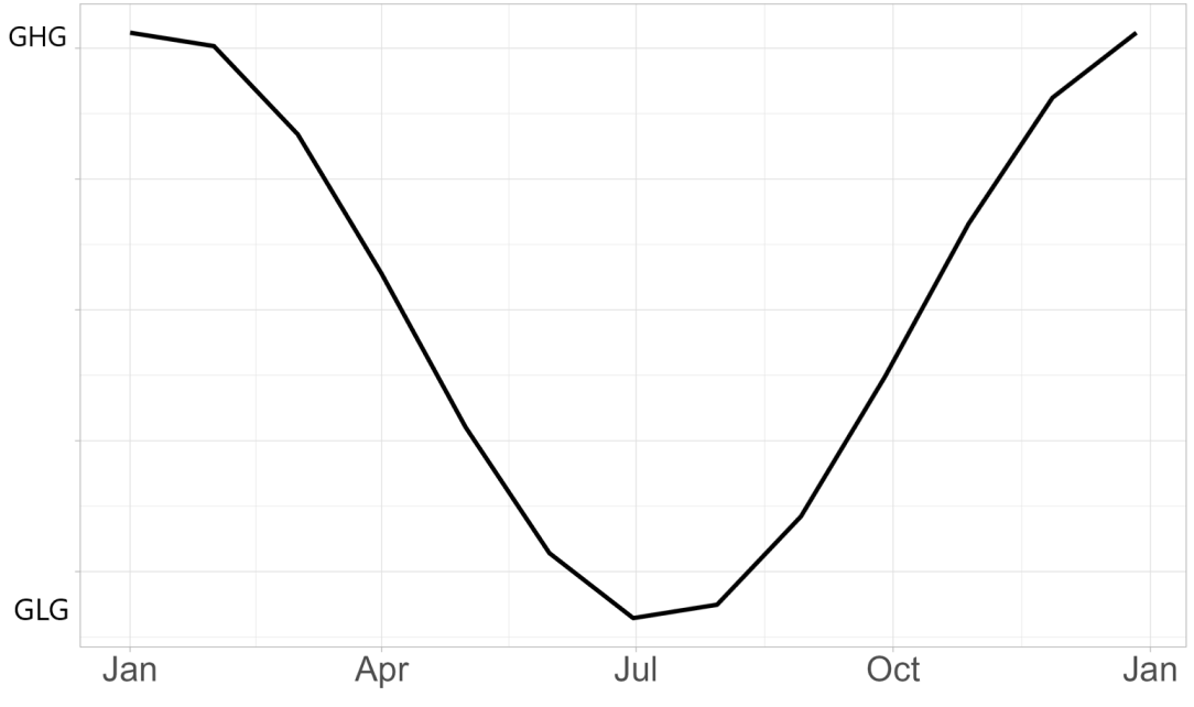
Figure 10:Average groundwater regime approximated with the sinus function based on the GHG and GLG.
Since GHG & GLG maps were developed assuming some correlation between precipitation, evapotranspiration and GWL, defining the locations where this correlation occurs is also important in order to use adequately the information available. Areas which depict some correlation could be modeled using the sinus function based on GHG and GLG, while areas without correlation could be simply modeled with the average groundwater levels.
Therefore, a correlation analysis was done to identify said areas. For this purpose, groundwater levels observations (2732) were downloaded from DOV using the python package pydov. These observations were compared with the monthly precipitation deficit (P-ET0), according to their specific location. The results of the correlation analysis and location of these observations in Flanders is shown in Figure 11. Locations showing some correlation (>0.25), have GWL mostly shallower than 3 m (depicted in orange). Therefore, the sinus function was used just in these locations, where the average GWL was shallower than 3 m.
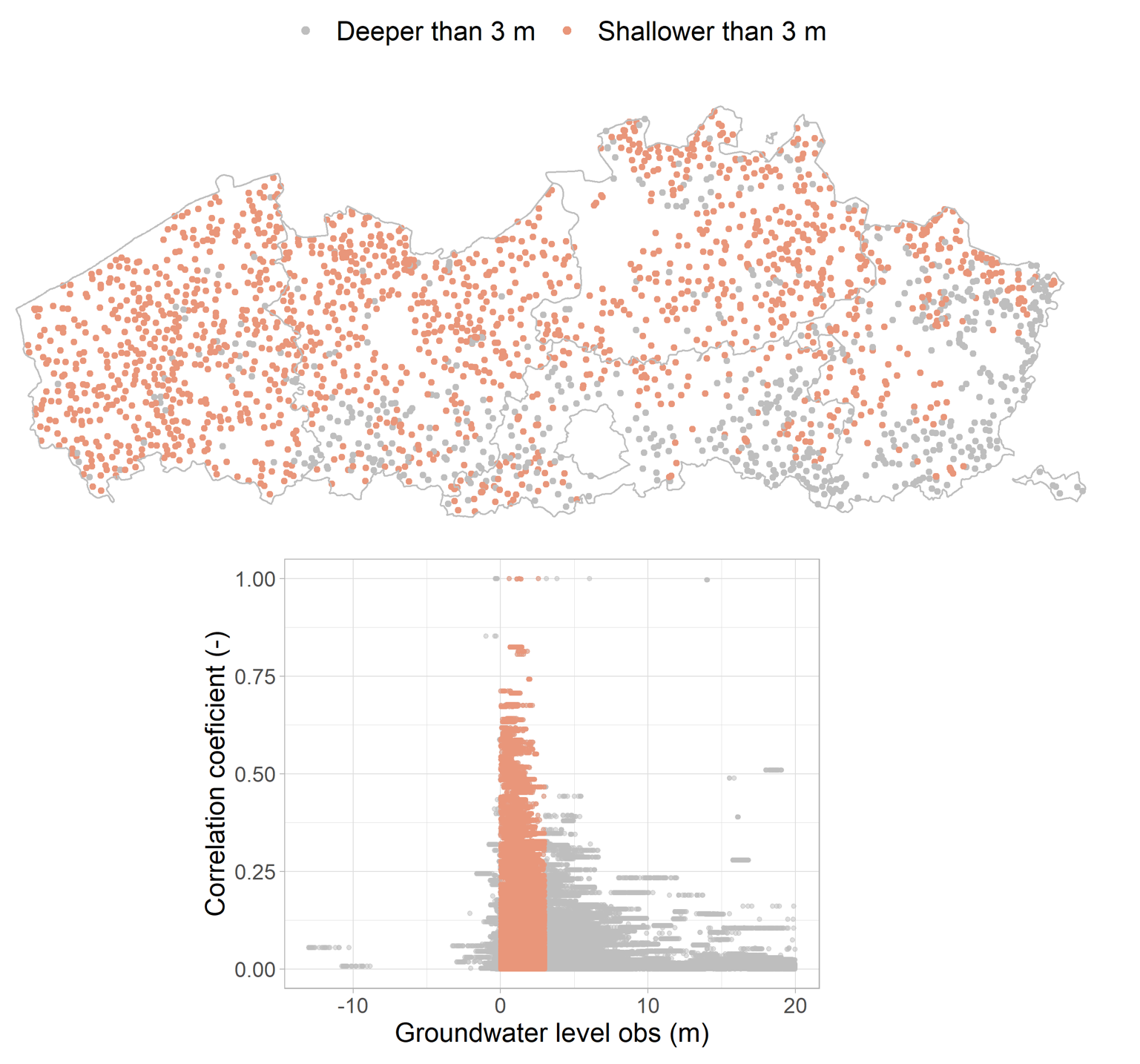
Figure 11:Correlation between precipitation deficit and groundwater levels. GWL shallower than 3 m are depicted in orange. Positive groundwater levels are below the soil surface.
Groundwater levels (GWL) served as bottom boundary condition in the model. GWL were converted to pressure heads in order to use the option 5 in SWAP. Pressure heads were obtained based on the reference located at 600 cm depth, which is the extent of the soil profile.
Model setup and running
Model running and analysis of model simulations involved three main steps, which are illustrated in Figure 12.
- Input data generation
- Model run
- Postprocessing
In synthesis, the model needs three main input files: meteo files (.met), crop files (.crp) and the main swap file (.swp). These files are supplied with information from the Sqlite database. The model runs using the model executable and these input files. The file “result_output.csv” is the main output of the model, that contains output variables like daily crop transpiration and biomass, which is previously defined in the sqlite database. During postprocessing, the potential and actual dry matter yield for each year, and yield reduction due to water stress and/or indirect effects are calculated.
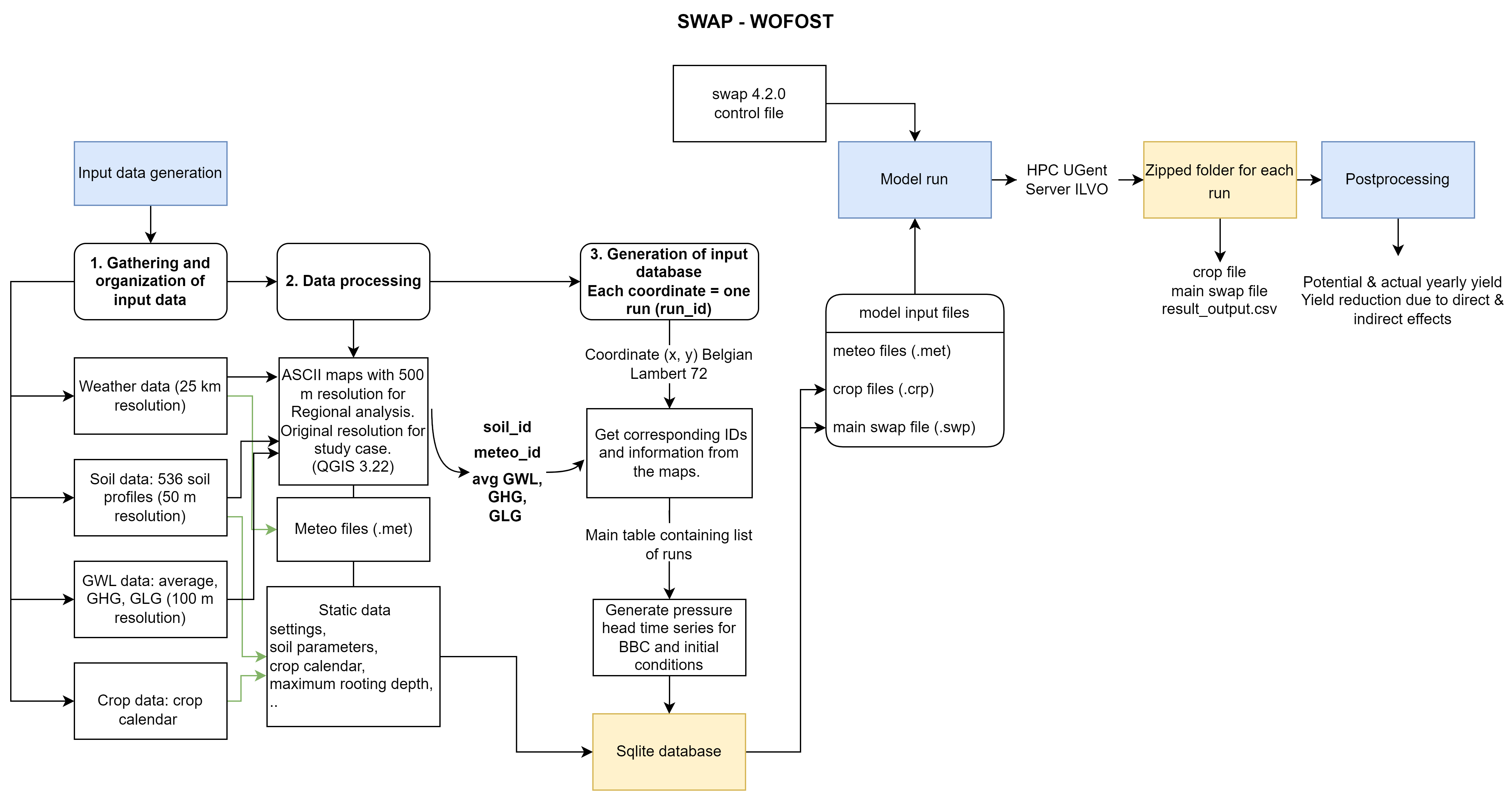
Figure 12:Flowchart of the input data generation, model run and model results processing using SWAP-WOFOST.
The first step to run the model is the generation of input data. The structure of the input data folders is showed in Figure 13. The crop folder contains the crop files (.crp), where detailed crop parameters for simulating crop growth and biomass assimilation are specified. The file location.csv has the coordinates (in Belgian Lambert 72) of every location where the model will be run. The input_data folder comprises most of the input data for each run, such us soil parameters, crop management parameters, and other input variables, which are stored in the Sqlite database. The maps folder contains the ASCII maps for meteo and soil IDs, and average GWL, GHG and GLG values. This information is also included in the database. Sqlite databases are then saved in the folder database. Five main Sqlites databases were created for each crop type, assuming that each crop covers the whole area.
The meteo folder holds the weather time series for each 25 x 25 m grid, in the correct format (.met), and CO2 emissions (.co2) until 2021. The source folder contains the model executable, version 4.2.0. The folders libraries and R scripts have the R libraries and R scripts for generating the databases and running the model.
The swap.swp file is the main swap file, containing general information regarding simulation, meteorology, crop rotation, irrigation, soil water flow, heat flow and solute transport. The main swap file draws the required information from the sqlite database. The control file control.inp contains directories and paths of the input data files.
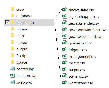
Figure 13:Organization of input data folders for running SWAP-WOFOST.
The next step involves running the model. This can be done directly in R studio or through a batch file. For the Regional analysis, simulations were executed in the UGent Super computer and/or the ILVO server. In the regional analysis, each simulation corresponds to a grid cell with 500 m resolution. In the case-study, each simulation corresponds to the center of an agricultural parcel.
The model output is available in a zipped folder containing the crop file, the main SWAP file and the result_output.csv file. The result_output.csv file contains the daily simulated potential and actual transpiration, transpiration reduction due to dry and wet conditions, potential and actual yield, and groundwater levels.
The final step is the postprocessing of the model results, where the yearly yields and total yield reduction due to direct (i.e. water stress) and indirect effects, and average GHG and GLG are determined.
The model instruments and general input data layers for Flanders can be freely downloaded from the PEILIMPACT github repository.
- Heinen, M., Mulder, M., & Kroes, J. (2021). SWAP 4 : technical addendum to the SWAP documentation [Techreport]. Wageningen Environmental Research. 10.18174/540451
- Mulder, M., Meijninger, W., & Broeke, M. (2021). Validatie waterwijzer landbouw: vergelijking modelresultaten Groenmonitor, Gram en Help. Stichting Toegepast Onderzoek Waterbeheer (STOWA).
- Kroes, J. G., Dam, J. C., Bartholomeus, R. P., Groenendijk, P., Heinen, M., Hendriks, R. F. A., Mulder, H. M., Supit, I., & Van Walsum, P. E. V. (2017). Swap version 4: Theory description and user manual (p. 248) [Techreport]. Wageningen Environmental Research. https://edepot.wur.nl/416321
- Werkgroep Waterwijzer Landbouw. (2018). Waterwijzer Landbouw: Instrumentarium voor kwantificeren van effecten van waterbeheer en klimaat op landbouwproductie (P. van & W. W. Landbouw, Eds.). http://edepot.wur.nl/464525
- van Dam, J. C., Groenendijk, P., Hendriks, R. F. A., & Kroes, J. G. (2008). Advances of Modeling Water Flow in Variably Saturated Soils with SWAP. Vadose Zone Journal, 7(2), 640–653. 10.2136/vzj2007.0060